

How To Draw Phase Diagram From Cooling Curve
Phase Diagrams and Solidification (all content)
Notation: DoITPoMS Teaching and Learning Packages are intended to be used interactively at a computer! This print-friendly version of the TLP is provided for convenience, but does non brandish all the content of the TLP. For case, any video clips and answers to questions are missing. The formatting (page breaks, etc) of the printed version is unpredictable and highly dependent on your browser.
Contents
Principal pages
Additional pages
Aims
On completion of this TLP you should:
- understand the thermodynamic principles backside free-energy curves
- understand how free-energy curves relate to equilibrium phase diagrams
- be able to construct a binary stage diagram from cooling curves
- be able to utilize stage diagrams to predict the composition and volume fraction of phases
Introduction
The phase diagram is a crucial office of metallurgy - information technology shows the equilibrium states of a mixture, so that given a temperature and composition, information technology is possible to calculate which phases volition be formed, and in what quantities. Every bit such information technology is very valuable to be able to construct a phase diagram and know how to use it to predict behaviour of materials.
The main theory behind phase diagrams is based around the latent oestrus that is evolved when a mixture is cooled, and changes phase. This means that past plotting graphs of temperature against time for a diversity of dissimilar compositions, it should be possible to see at what temperatures the unlike phases class.
It is relatively easy to produce a rough binary phase diagram, as will be shown later in the package, simply although it is quick to have readings for the top role of a phase diagram, it takes longer, and hence more sensitive equipment to monitor the changes that take place when a solid changes stage. A typical simple binary stage diagram is every bit follows:
Where 50 stands for liquid, and A and B are the two components and α and β are two solid phases rich in A and B respectively. The blue lines represent the liquidus and solidus lines, which are relatively simple to measure. The ruby-red lines involve a solid-to-solid transition, and so crave much more sensitive equipment.
Nonetheless, there is also a lot of thermodynamic theory backside stage diagrams, which allows more problematic or more complex systems to exist predicted, and this can lead to faster cosmos of phase diagrams, as it can take a long time to pick up all the stable phases in experiments, and in that location is not always the time available for such practical work.
A crucial point to recollect is that a phase diagram should e'er display the equilibrium phases, and and so with libation temperatures, these are hard to reach due to kinetic problems. Even at higher temperatures, there may be issues of having enough time for the solid to fully equilibrate as the system is cooling.
Thermodynamics: Basic terms
Internal Free energy, U
The internal energy of a organization is the sum of the potential free energy and the kinetic energy. For many applications it is necessary to consider a small alter in the internal energy, dU, of a organization.
dU = dq + dw = CdT - PdV
dq = the heat supplied to a organization
dw = the work performed on the system
C = heat capacity
dT = change in temperature
P = pressure level
dV = modify in book
At constant volume,
dU = C 5 dT
Enthalpy, H
Enthalpy is the constant pressure version of the internal energy. Enthalpy,
H = U + PV.
Therefore, for small changes in enthalpy,
dH = dU + PdV + VdP.
At constant pressure level,
dH = CPdT.
Entropy, Due south
Entropy is a measure of the disorder of a system. In terms of molecular disorder, the entropy consists of the configurational disorder (the system of different atoms over identical sites) and the thermal vibrations of the atoms about their mean positions. A change in entropy is divers as,
\[dS \ge \frac{{{\rm{d}}q}}{T}\]
For reversible changes, i.east. changes nether equilibrium atmospheric condition,
dq = TdS
For natural changes, i.e. under non-equilibrium conditions,
dq < TdS
Gibbs costless energy, G
The Gibbs free energy can exist used to ascertain the equilibrium state of a arrangement. Information technology considers only the properties of the system and not the backdrop of its surroundings. It can be thought of equally the free energy which is bachelor in the arrangement to do useful work.
Free energy, G, is divers as,
G = H - TS = U + PV - TS
For pocket-sized changes,
dG = dH - TdS - SdT = VdP - SdT + (dq - TdS)
For changes occurring at constant pressure and temperature,
dG = dq - TdS
Therefore, dG = 0 for reversible (equilibrium) changes, and dG < 0 for non-reversible changes.
From this it is clear that M tends to a minimum at equilibrium.
The Helmholtz free energy, F, is sometimes used instead of G, and is the equivalent of Grand for changes at constant volume. It is defined as,
F = U - TS
Thermodynamics of Solutions
Consider a mechanical mixture of ii phases, A and B. If this is so transformed into a single solution phase with A and B atoms distributed randomly over the diminutive sites, and so there will be,
- An enthalpy change associated with interactions between the A and B atoms, ΔH mix
- An entropy change, ΔS mix, associated with the random mixing of the atoms
- A free energy of mixing, ΔOne thousand mix = ΔH mix - TΔS mix
Presume that the organization consists of North atoms: x A Northward of A and x B Northward of B, where,
ten A = fraction of A atoms and x B = (1 - 10 A) = fraction of B atoms
Enthalpy of mixing
In calculating ΔH mix information technology is assumed that only the potential energy term undergoes whatsoever significant change during mixing. This change arises from the interactions between nearest-neighbor atoms. Consider an alloy consisting of atoms A and B. If the atoms adopt similar neighbours, A atoms volition tend to cluster and likewise B atoms, and so a greater number of A-A and B-B bonds will form. If the atoms prefer unlike neighbours a greater number of A-B bonds will class. If there is no preference A and B atoms will exist randomly distributed.
Let w AA be the interaction free energy betwixt A - A nearest neighbours, w BB that for B - B nearest neighbours and w AB that for A - B nearest neighbours.
All of these energies are negative, as the zilch in potential free energy is for infinite separation between atoms.
Let each cantlet of A and B have co-ordination number z.
Therefore, the full number of nearest-neighbour pairs is Nz/2.
Probability of A - A neighbours = x A ii
Probability of B - B neighbours = x B two
Probability of A - B neighbours = 2x A x B
For a solid solution the full interaction free energy is,
H south - U south = Nz/2 (x A two due west AA + x B 2 westward BB + ii10 A 10 B west AB)
For pure A, H A = (Nz/2)w AA
For pure B, H B = (Nz/2)w BB
Hence the enthalpy of mixing is given by,
ΔH mix = H s - (x A H A + x B H B) = (Nz/2)10 A 10 B (iiwestward AB - w AA - westward BB)
We can define an interaction parameter
W = (Nz/two)(iiwest AB - west AA - westward BB)
Therefore,
ΔH mix = Westward x A x B
If A-A and B-B interactions are energetically more favourable than A-B interactions then W > 0. Then, ΔH mix > 0 and there is a tendency for the solution to grade A-rich and B-rich regions.
If A-B interactions are energetically more favourable than A-A and B-B interactions, W < 0, ΔH mix < 0, and at that place is a trend to form ordered structures or intermediate compounds.
Finally if the solution is ideal and all interactions are energetically equivalent, then W = 0 and ΔH mix = 0.
Entropy of mixing
Per mole of sites, this is
ΔS mix = kN (- x Alnten A - x Blnx B)
(the derivation of this effect makes use of Stirling'south approximation)
where N = Avogadro's number, and kN = R, the gas abiding.
Hence,
ΔSouthward mix = R (- 10 Alnx A - ten Blnten B)
A graph of ΔS mix versus x A has a different course from ΔH mix. The curve has an infinite gradient at x A = 0 and x A = 1.
The gratuitous free energy of mixing is now given by,
ΔChiliad mix = ΔH mix - TΔSouth mix = x A ten B W + RT (10 A lnx A + x Blnx B)
For W < 0, ΔG mix is negative at all temperatures, and mixing is exothermic. For W > 0, ΔH mix is positive and mixing is endothermic.
Free energy curves
For whatsoever phase the energy, G, is dependent on the temperature, pressure and composition.
Pure Substances
For pure substances the composition does not vary and at that place is little dependence on pressure. Therefore the free energy varies greatest with temperature.
The phase with the lowest gratuitous energy at a given temperature will be the most stable. The curves for the gratuitous energies of the liquid and solid phases of a substance have been plotted beneath. It shows that beneath the melting temperature the solid stage is nigh stable, and in a higher place this temperature the liquid phase is stable. At the melting temperature, where the two curves cantankerous, the solid and liquid phases are in equilibrium.
Solutions
Solutions contain more than one component and in these situations the free energy of the solution will go dependent on its composition as well as the temperature.
It is shown above that the gratis energy of mixing is:
Δ G mix = Δ H mix - T Δ S mix = x A ten B W + RT (x A lnx A + x Bln10 B)
The shape of the Δ G mix curve is dependent on temperature . For the bend shown below the value of Δ H mix is positive, leading to a maximum on the curve at low temperatures. Δ Thou mix is ever negative for low solute concentrations equally the gradient of Δ South mix is infinite at x A = 0 and x A = 1.
At high temperatures at that place is a complete solution and the curve has a single minimum. At low temperatures the curve has a maximum and 2 minima. In the limerick range between the ii minima (denoted by the dashed lines) a mixture of ii phases is more stable than a unmarried-phase solution.
The costless energy of a regular solid solution, Δ One thousand sol, is the sum of the free energy of mixing Δ G mix and the gratuitous free energy of fusion Δ Grand fus.
Gratuitous energy of fusion
When a liquid solidifies there is a alter in the gratis energy of freezing, as the atoms movement closer together and form a crystalline solid. For a pure component, this tin be empirically calculated using Richard's Dominion:
Δ 1000 fusion = - ix.5 (T m - T)
T m = melting temperature
T = current temperature
Δ G fusion = 0 at the melting temperature of the component.
Δ G fusion < 0 below the melting temperature of the component.
Δ Thou fusion > 0 above the melting temperature of the component.
In an alloy, if both the liquid and solid solutions are platonic then Δ G fusion for the blend tin can be interpolated between the values for the 2 components.
Now we can plot the complimentary energy of a regular solid solution from the equation,
Δ G sol = Δ G mix + Δ Chiliad fusion
Phase diagrams 1
Costless energy curves can be used to decide the most stable country for a system, i.e. the stage or phase mixture with the lowest free energy for a given temperature and composition. Below is a schematic costless-energy curve for the solid phase of an blend.
The solid shown could either be as a mixture or equally a homogeneous solution of A and B. The figures below prove that an alloy of composition C tin exist in different configurations with differing free energies. In the first figure (below) the energy of unmixed A and B is shown equally the diagonal black line. The gratuitous free energy of this mixture at composition C is shown as a ruby-red point.

The arrangement can reduce its free energy by existing as a mixture of 2 phases
Though the system has reduced its gratis energy from that of the mixture, the most stable configuration for the organization is a solid solution. This allows the free free energy of the system to sit on the gratuitous energy curve.
For most systems there will be more than one phase and associated free-energy curve to consider. At a given temperature the most stable phase for a system can vary with limerick. While the system could consist entirely of the phase which is most stable at a given composition and temperature, if the free free energy curves for the two phases cross, the virtually stable configuration may be a mixture of two phases with compositions differing from that of the overall system. The total energy of the system in whatever given two-phase configuration tin can be found by linking the two phases in question with a straight line on a free-free energy plot.
Taking a line that is a common tangent to the 2 costless-energy curves produces the lowest possible gratis energy for the arrangement as a whole. Where the line meets the gratuitous energy curves defines the composition of each phase.
For positions where it is not possible to draw a common tangent between the two free-energy curves the organisation volition sit down entirely in the stage with the lowest free free energy. The borders between the single- and two-phase regions mark the positions of the solidus and liquidus on the phase diagram.
When the temperature is altered the compositions of the solid and liquid in equilibrium change and build up the shape of the solidus and liquidus curves on a phase diagram.
Below, a binary system can exist seen along with the gratis-free energy curves for the liquid and solid phases at a range of temperatures shown on the phase diagram.
Phase diagrams ii
The gratuitous-free energy curves and stage diagrams discussed in Phase Diagrams 1 were all for systems where the solid exists every bit a solution at all compositions and temperatures. In near real systems this is not the instance. This is due to a positive Δ H mix caused by unfavourable interactions between dissimilar neighbour atoms. As the temperature is reduced the Δ H mix term becomes more significant and the curve turns upward at intermediate compositions, resulting in a curve with 2 minima and 1 maximum equally described earlier. A mutual tangent tin can and so exist fatigued between the two minima showing that the system can reduce its costless free energy through existing as a mixture of ii distinct phases.
The complimentary free energy of a organisation of composition Co tin be minimised by existing as a mixture of ii solid phases of composition Ci and C2:
This consequence can result in a arrangement which, though single-phase upon solidification, will separate into ii solid phases on cooling (e.g. Cr-W).
Another possible result is that the complimentary-energy bend for the liquid will intersect the up turned section of the free-energy curve for the solid before the temperature is high enough to induce the formation of a solid solution. Equally the temperature is increased, the gratis-energy curve for the liquid moves downwardly relative to the solid curve and reaches a position where it is possible to link two parts of the solid free free energy curve and one part of the liquid free energy curve with a mutual tangent. At this temperature three phases are in equilibrium.
Here the system is at the eutectic temperature and three phases can exist joined past a common tangent:
This is known as the eutectic temperature. At this temperature there will exist a composition which solidifies at a single temperature through the co-operative growth of the two solid phases. This is the eutectic composition. It is this composition which will exhibit the lowest melting point for the system.
At temperatures above that of the eutectic there will be two common tangents producing two two-phase regions at the same temperature. The two different solid phases are normally labeled equally α and β
Eutectic systems therefore have a liquidus which contains a 5 to the eutectic point where it meets the eutectic invariant-reaction line.
Hither is an instance of a eutectic phase diagram. α and β are both solid phases.
The two-phase solid region on the phase diagram volition consist of a mixture of eutectic and either α or β phase depending on the whether the alloy composition is hypoeutectic or hypereutectic. The constitution of an blend under equilibrium conditions can be found from its stage diagram. This will exist discussed in a afterwards department.
Interpretation of cooling curves
The melting temperature of any pure material (a one-component arrangement) at constant pressure level is a single unique temperature. The liquid and solid phases exist together in equilibrium only at this temperature. When cooled, the temperature of the molten material volition steadily decrease until the melting betoken is reached.
At this point the material will start to crystallise, leading to the evolution of latent heat at the solid liquid interface, maintaining a constant temperature across the material. Once solidification is complete, steady cooling resumes. The abort in cooling during solidification allows the melting point of the material to be identified on a time-temperature curve.
Most systems consisting of two or more components exhibit a temperature range over which the solid and liquid phases are in equilibrium. Instead of a single melting temperature, the system at present has two different temperatures, the liquidus temperature and the solidus temperature which are needed to describe the change from liquid to solid.
The liquidus temperature is the temperature in a higher place which the organization is entirely liquid, and the solidus is the temperature below which the system is completely solid. Between these two points the liquid and solid phases are in equilibrium. When the liquidus temperature is reached, solidification begins and there is a reduction in cooling rate caused past latent rut evolution and a consequent reduction in the gradient of the cooling curve.
Upon the completion of solidification the cooling rate alters again assuasive the temperature of the solidus to be adamant. Equally tin be seen on the diagram beneath, these changes in gradient allow the liquidus temperature T L, and the solidus temperature T S to be identified.
When cooling a fabric of eutectic composition, solidification of the whole sample takes place at a unmarried temperature. This results in a cooling curve similar in shape to that of a unmarried-component organization with the organisation solidifying at its eutectic temperature.
When solidifying hypoeutectic or hypereutectic alloys, the first solid to form is a single stage which has a composition dissimilar to that of the liquid. This causes the liquid composition to arroyo that of the eutectic as cooling occurs. Once the liquid reaches the eutectic temperature it volition take the eutectic composition and volition freeze at that temperature to class a solid eutectic mixture of two phases.
Formation of the eutectic causes the system to cease cooling until solidification is consummate. The resulting cooling curve shows the ii stages of solidification with a section of reduced gradient where a unmarried phase is solidifying and a plateau where eutectic is solidifying.
By taking a series of cooling curves for the same system over a range of compositions the liquidus and solidus temperatures for each composition can be determined assuasive the solidus and liquidus to be mapped to determine the stage diagram.
Below are cooling curves for the same system recorded for dissimilar compositions and and so displaced along the time axis. The ruby regions indicate where the fabric is liquid, the blue regions signal where the material is solid and the greenish regions indicate where the solid and liquid phases are in equilibrium.
By removing the time axis from the curves and replacing it with composition, the cooling curves point the temperatures of the solidus and liquidus for a given composition.
This allows the solidus and liquidus to be plotted to produce the phase diagram:
Experiment and results
The simplest style to construct a phase diagram is past plotting the temperature of a liquid against time as it cools and turns into a solid. As discussed in Interpretation of cooling curves, the solidus and liquidus can be seen on the graphs as the points where the cooling is retarded past the emission of latent oestrus.
Method
An experiment tin can exist performed to go a rough idea of a phase diagram by recording cooling curves for alloys of two metals, in various compositions. The alloy called for this example is bismuth-tin can, both of which metals accept low melting points, and then can be heated and cooled more quickly and easily in the lab. So that the experiment could be performed in a reasonable fourth dimension, 11 compositions were used, from pure bismuth to pure tin can in steps of 10%. All the compositions were measured in weight percent.
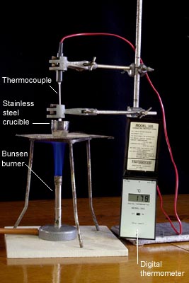 | 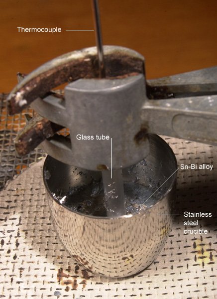 |
| Heating apparatus | Crucible |
| (Click on image to view a larger version) | |
The appliance pictured was fix, with the maximum temperature to be attained of effectually 300°C. The sample in the crucible cooled, and the temperature was recorded at regular intervals. In the case of the results produced hither, readings were made every two seconds, using a estimator. Yet, it is adequate to take readings every fifteen seconds manually.
Results
The process was repeated for all 11 compositions, and the following results recorded:
These lines can be made clearer past spacing them along the time axis, so that the alloys with a higher bismuth content announced further to the right, as shown below.
From these graphs it is possible to pick out the changes in slope which permit a simplified phase diagram to be drawn.
On the diagram with the displaced time-temperature plots, the changed gradients, i.e. the parts where some of the liquid is solidifying, are coloured white. These show the acme of the liquidus and the bottom of the solidus.
If these curves are now straightened out, and the colours kept, with the white representing the solidification, it is possible to construct a basic phase diagram, as was shown for an isomorphous system in Estimation of cooling curves. This is shown below, where the white line is part of the phase diagram, constructed from the cooling curves, and the thin greyness line is the bodily phase diagram, found from many experiments over a long period of time.
Analysis
It can be seen from the diagram above that the recorded stage diagram is roughly 15°C lower than it should be, and that some of the measurements of the liquidus are non in the expected places. The lowering of the diagram is due to the thermocouple being contained in a glass rod, rather than actually touching the blend. The occasional unexpected liquidus temperatures are probably due to the compositions being slightly inaccurate.
It is also worth noting that in this projected phase diagram, it was non possible to describe in a proper solidus on the correct hand side, as none of the compositions most pure bismuth showed bear witness of a solidus. As such, a dotted line has been plotted equally an approximate of where it would go.
The microstructure of the alloy changes with composition. This can be seen in scanning electron microscope (SEM) images taken from each of the compositions used in the experiment above.
Interactive Sn-Bi phase diagram and SEM images
The lever rule
If an alloy consists of more than one phase, the amount of each stage present tin can be constitute past applying the lever rule to the phase diagram.
The lever rule tin can be explained by because a simple balance. The composition of the alloy is represented past the fulcrum, and the compositions of the ii phases by the ends of a bar. The proportions of the phases nowadays are determined by the weights needed to residue the system.
And then,
fraction of phase 1 = (C2 - C) / (C2 - Cane)
and,
fraction of phase 2 = (C - C1) / (Cii - C1).
Lever rule applied to a binary arrangement
Point ane
At point 1 the blend is completely liquid, with a composition C. Allow
C = 65 weight% B.
Point 2
At indicate 2 the blend has cooled as far equally the liquidus, and solid phase β starts to form. Phase β showtime forms with a composition of 96 weight% B. The green dashed line below is an case of a necktie-line. A tie-line is a horizontal (i.east., constant-temperature) line through the chosen point, which intersects the phase purlieus lines on either side.
Point 3
A tie-line is drawn through the signal, and the lever dominion is applied to identify the proportions of phases present.
Intersection of the lines gives compositions Cane and C2 every bit shown.
Let
C1 = 58 weight% B
and
Ctwo = 92 weight% B
So,
fraction of solid β = (65 - 58) / (92 - 58) = 20 weight%
and
fraction of liquid = (92 - 65) / (92 - 58) = 80 weight%
Point 4
Allow
C3 = 48 weight% B
and
C4 = 87 weight% B
So
fraction of solid β = (65 - 48) / (87 - 48) = 44 weight%.
As the blend is cooled, more solid β phase forms.
At signal four, the balance of the liquid becomes a eutectic phase of α+β and
fraction of eutectic = 56 weight%
Point five
Let
C5 = 9 weight% B
and
Cvi = 91 weight% B
So
fraction of solid β = (65 - 9) / (91 - nine) = 68 weight%
and
fraction of solid α = (91 - 65) / (91 - nine) = 32 weight%.
Modern uses
Phase diagrams are not just an abstract construction - they accept applications in the real world, in deciding which compositions to use.
A major utilize of eutectics, or near eutectics is in solder. In plumbing, solder is used to join copper pipes together, producing a waterproof seal. For many years a atomic number 82-tin alloy has been used, as this has a low melting point, especially at eutectic. However, although a low melting point is sought, information technology is useful to be able to move the pipes around slightly when they are in place and the solder is solidifying. This means that a eutectic should non be used, as although information technology has the lowest melting signal for the blend system, it will all solidify at once, leaving little room for error. Instead information technology is useful to employ an alloy whose limerick deviates slightly from that of the eutectic, so that the solidification will take longer, making the solder easier to employ, despite the college temperatures, and then resulting in a meliorate join.
Electric solder uses a similar alloy to join parts of an electronic circuit together. In the instance of a standard electrical solder, the eutectic is used, as loftier temperatures are to exist avoided, and information technology is useful for the solder to solidify all at one time.
In more modern soldering applications, such equally a ball grid assortment which joins the fleck to some circuit boards, the eutectic is still used. However, there are too situations where a slightly off-eutectic tin can be used. If there are several processing steps, it is useful to outset off with a college melting point alloy, and only use the eutectic in the last soldering stage. This allows the previous solders to stay in place when the heating takes place on the later stages.
Modern solders have moved away from pb-based alloys, because of environmental considerations, and been replaced with new alloys. In the case of plumbing, there is a tendency to use plastic piping instead of copper piping, and so in that location is less need for solder in this manufacture. In the electronics industry, atomic number 82-tin is beingness replaced by copper-, tin can-, and silver-based systems, which accept less environmental problems, only can still be used to create low melting points and flexibility which the lead-tin systems provide. Lots of the modern enquiry on solders relates to alternative systems, and characterising them for utilize. Part of this characterisation involves the product of phase diagrams to allow good option of limerick for the right backdrop.
In recent times, it has become necessary to mix several elements in order to better properties of the materials. It is therefore useful to create phase diagrams which involve iii elements, chosen "ternary" diagrams. These are more complicated than two chemical element "binary" stage diagrams, but allow improved optimisation, and hence tin produce amend results.
Farther considerations
Other methods for constructing phase diagrams
Although the easiest mode to investigate stage transformations is by the utilise of time temperature cooling curves, in that location are many ways to investigate these changes. This is most helpful when observing solid to solid stage changes, as these take longer to reach equilibrium, and and so the cooling of a textile must have place at a slower rate in guild to go accurate results. Unfortunately, every bit the rate of cooling decreases, information technology gets harder to discover the latent heat existence released, and then other methods must be sought.
The thinking behind almost of the methods is the aforementioned; as the material changes phase, there will exist changes in its physical properties. As such, the phase modify tin be detected by observing a belongings as the temperature is reduced. Examples of this are density, electric or thermal resistance, optical properties, Young's modulus and damping efficiency. Another oft used measure out is that of interplanar spacings in the crystalline phases, which can be measured using 10-ray diffractometry.
These techniques have been used to map out phase diagrams, just they are ever time consuming, specially during the solid transformations.
Dangers in interpretation of phase diagrams
An essential bespeak to recall in stage diagrams is that during normal or fast cooling, results may not be as expected in the diagram. Both the theory and the experiments to construct stage diagrams rely on the assumption that the organization is in equilibrium, which is rarely the case, equally this merely occurs properly when the system is cooled very slowly. In lodge to reach full equilibrium, the solute in the solid phases must stay completely uniform throughout the cooling. However, in most systems, if the organization is not cooled quickly, the phase diagram will give fairly accurate results. In addition, nearly the eutectic, the results become even closer to the phase diagram, equally the liquid solidifies at nearly the same time.
The non equilibrium conditions tin can sometimes exist of benefit yet, as microstructures at higher temperatures in a stage diagrams may sometimes be preserved to lower temperatures by fast cooling, i.e. quenching, or unstable microstructures may occur during fast cooling which can be useful when hardening an alloy.
Summary
In this package, the theoretical background to phase diagrams has been shown, likewise as a method for constructing role of a diagram. Explanation has been given of how to utilize a phase diagram, and how it applies to real systems, and to agreement solidification.
It should now be appreciated that phase diagrams are a valuable resource in predicting behaviour of alloys during solidification, and the microstructures which will exist produced.
However, there should too exist an understanding that in normal cooling conditions although phase diagrams are more often than not fairly accurate, they are not always verbal, and if improvidence is slow, there may exist unexpected results.
Questions
Quick questions
You should be able to respond these questions without as well much difficulty after studying this TLP. If non, then y'all should become through it again!
-
What is the effect on the shape of the free-energy curve for a solution if its interaction parameter is positive?
-
In terms of interatomic bonding, what does a negative interaction parameter represent?
-
Cooling curve for a binary system:
-
What is a hypoeutectic alloy?
-
Await at the following Al-Si phase diagram. (Identify the mouse over the diagram to determine the temperature and composition at whatsoever betoken.)
For an Al five wt% Si alloy what volition exist the composition of the solid in equilibrium with the liquid at 600�C?
-
Expect at the following Cu-Al phase diagram. (Place the mouse over the diagram to determine the temperature and composition at any point.)
What will be the relative weight fraction of CuAl2 (θ) in a Al 15wt% Cu alloy at its eutectic temperature?
Deeper questions
The following questions require some thought and reaching the respond may require you to recall beyond the contents of this TLP.
-
Using the following data, calculate the volume fraction of the beta phase and eutectic at the eutectic temperature, for an alloy of composition 75 wt% Ag. Assume equilibrium weather.
At eutectic temp:
eutectic composition = 71.nine wt% Ag
maximum solid solubility of Cu in Ag = 8.viii wt% Cu
density Ag = x 490 kg/mthree
density Cu = 8 920 kg/m3
-
Composition vs temperature phase diagrams exist for the combinations of three elements A, B and C (i.e. the three stage diagrams A-B, A-C and B-C). How might they exist arranged in three-dimensional space to construct a "ternary" phase diagram for a system containing A, B and C?
Open-ended questions
The following questions are not provided with answers, simply intended to provide food for thought and points for further word with other students and teachers.
-
Nether what conditions could the compositions of the phases present differ from that predicted in the phase diagram?
Going further
Books
- Porter, D. A. and Easterling K, Phase Transformations in Metals and Alloys, 2nd edition, Routledge, 1992.
- Smallman, R. Due east, Modernistic Physical Metallurgy, Butterworth, 1985.
- John, V, Understanding Phase Diagrams, Macmillan,1974.
Websites
- Alloys and their phase diagrams - including examples of Binary Isomorphous Alloy Systems
An Adobe Acrobat file authored by Professor P.J.K. Monteiro at the University of California, Berkeley. - Solidification
A MATTER module with storyboard past Professor Neb Clyne providing an in-depth look at processes involved in solidification.
Stirling's approximation
Stirling's approximation is:
ln Northward! = NlnN -N, for big N
The entropy,
South = m lnw
where due west is the number of possible configurations for a organization.
For a mechanical mixture w = 1 as the only organization is A atoms on A sites and B atoms on B sites.
For a solid solution of A and B containing 10 A N A atoms and x B N B atoms the value of w is calculated every bit follows
Bold that the thermal entropy of the organization remains unchanged when A and B go into solution
| ΔDue south mix | = |
| |||||
| = | k [ln N! - ln {ten A N}! - ln {(1 - x A)North}!] | ||||||
| = | k [ North ln N - N - x A N ln x A Due north + ten A Northward - (1 - x A)Northward ln (1 - x A)North + (ane - x A)N] | ||||||
| = | kN [ln N - one - 10 A ln ten A N + ten A - (1 - x A) ln (i - x A)N + (1 - x A)] | ||||||
| = | kN [ln N - x A ln {x A North} - (ane - 10 A) ln {(ane - x A)N}] | ||||||
| = | kN [ln N - x A ln x A - x A ln North - (i - x A) ln (one - x A) - ln N + x A ln Due north | ||||||
| = | kN [- x A ln x A - (1 - x A) ln (one - x A)] | ||||||
| = | kN [- ten A ln x A - x B ln x B] |
Academic consultant: Lindsay Greer (University of Cambridge)
Content evolution: Matt Charles, Jacqui Capes and Andrew Cockburn
Photography and video: Brian Barber and Carol Best
Spider web development: Dave Hudson
This TLP was prepared when DoITPoMS was funded by the Higher Education Funding Council for England (HEFCE) and the Department for Employment and Learning (DEL) under the Fund for the Development of Teaching and Learning (FDTL).
Boosted support for the development of this TLP came from the Armourers and Brasiers' Company and Alcan.

Source: https://www.doitpoms.ac.uk/tlplib/phase-diagrams/printall.php
Posted by: taylorcultin.blogspot.com
0 Response to "How To Draw Phase Diagram From Cooling Curve"
Post a Comment